
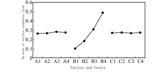
In the metal cutting process, cutting force is an important physical quantity, and surface roughness is one of the important indicators to measure the quality of processing. Accurate prediction of cutting force and surface roughness has a positive effect on cutting. It can be seen from the above test results that the cutting amount has a very obvious influence on the cutting force and surface roughness.
BP neural network is a feed-forward artificial neural network based on ErrorBack Propagation (BP). Its main features include nonlinear mapping capabilities, generalization capabilities, and fault tolerance. BP neural network is generally composed of input layer, output layer and several hidden layers. Among them, single hidden layer BP neural network is the most widely used. The essence of the learning algorithm of BP neural network is to obtain the minimum value of the total error of the network by correcting the weight of the error function in the negative gradient direction. The algorithm includes two processes of working signal forward propagation and error signal back propagation. This paper uses BP neural network prediction to predict the accuracy of cutting force and surface roughness.
(1) Sample grouping
The BP neural network can automatically use 15% of the 64 samples obtained from the full factor cutting test as the test group, and the remaining samples as the training group. The training group will be used to build the prediction model, and the test group's role is to verify the prediction accuracy of the prediction model.
(2) BP neural network structure design
1.Determine the number of nodes in the input layer and output layer
The relationship between cutting amount, cutting force and surface roughness is established through BP neural network. Therefore, the number of nodes in the input layer is 3, which are the back-grab ap, the feed amount f, and the cutting speed v; the number of nodes in the output layer is 4, which are radial force Fp, tangential force Fc, and axial force. Force Ff and surface roughness Ra.
2.Determine the number of hidden layers
According to the literature, all continuous functions can be mapped by a single hidden layer feedforward neural network. The functions of cutting force and surface roughness studied in this paper are continuous, so a hidden layer is designed first. If a hidden layer can not accurately establish the mapping relationship between the input set and the output set, only consider designing two hidden layers.
3.Determine the number of hidden layer nodes
Use trial and error method to determine the number of nodes in the hidden layer of the neural network, design the neural network in the order of the number of hidden layer nodes from less to more, use the same sample set to train each designed neural network, and train the network with the smallest error The number of hidden layer nodes corresponding to the structure is the optimal number of hidden layer nodes. The initial value of the trial and error method is generally determined by the following empirical formula,

In the formula, m is the number of hidden layer nodes; n is the number of input layer nodes; l is the number of output layer nodes; α is a constant between 1-10. According to formula (1) and formula (2), the initial value of this trial and error method is 3. Table 6 shows the neural networks and their mean square errors designed according to the trial and error method. Due to the randomness of the BP neural network algorithm, the results of each operation of the same network are different, so each network is trained 10 times, and the average of the mean square errors of the 10 training times is taken.
|
Number of hidden layer nodes |
3 |
4 |
5 |
6 |
7 |
8 |
|
Mean mean square deviation |
0.034 |
0.032 |
0.026 |
0.027 |
0.039 |
0.042 |
|
Number of hidden layer nodes |
9 |
10 |
11 |
12 |
13 |
|
Mean mean square deviation |
0.034 |
0.045 |
0.052 |
0.046 |
0.057 |
It can be seen from the table that as the number of hidden layer nodes increases, the mean square error of the network decreases first and then increases. When the number of nodes is 5, the mean square error of the network is the smallest, so the optimal number of hidden layer nodes Is 5.
4.Determine the transfer function of the hidden layer of the transfer function using a nonlinear hyperbolic tangent sigmoid (Tan-Sigmoid) transfer function, which can map the input value from (-∞, +∞) to (-1, 1) . The transfer function of the output layer uses a linear purelin function. The Sigmoid function is not used because the linear function can reduce the complexity of the calculation and avoid the output value being limited to (0, 1) or (-1, 1).
(3) Choice of optimization algorithm.
The standard BP algorithm to modify the weight method is the fastest gradient descent method. In practical applications, there are often shortcomings such as easy to fall into local minimums, easy to be affected by the order of samples, and slow convergence. Generally, the standard BP algorithm is not directly applied, but Optimize the standard BP algorithm.
Considering factors such as convergence speed, computing resources and network accuracy, the L-M method, conjugate gradient method and Bayesian regularization are selected to improve the BP algorithm respectively, and the results are shown in Table 7. Similarly, due to the randomness of the BP neural network algorithm, even if the optimization algorithm is the same, the results of each operation are different, so the network is trained 10 times under each optimization algorithm, and the average of the 10 training effects is calculated.
According to Table 7 to measure the network convergence speed and network accuracy, it is concluded that the optimization effect of the L-M algorithm is better. Therefore, the L-M algorithm is selected as the training algorithm of the BP neural network.
(4) Training results of BP neural network
According to the determined neural network structure and training algorithm, a cutting force prediction model based on BP neural network is constructed. The network divides the 54 input samples into training samples, verification samples, and test samples at a ratio of 70%, 15%, and 15%. Among them, the function of the training sample is to train the neural network, the verification sample is used to verify the generalization ability of the neural network, and the function of the test sample is to test the performance of the network. The network ends training when the generalization stops improving or the number of iterations reaches the upper limit.
|
Training times |
Levenberg-Marquardt |
Bayesian regularization |
conjugate gradient methods |
|||
|
Number of iterations |
Network mean square error |
Number of iterations |
Network mean square error |
Number of iterations |
Network mean square error |
|
|
1 |
14 |
0.0139 |
25 |
0.0175 |
61 |
0.0267 |
|
2 |
5 |
0.0169 |
52 |
0.0054 |
11 |
0.1850 |
|
3 |
13 |
0.0436 |
45 |
0.0176 |
46 |
0.0889 |
|
4 |
12 |
0.0567 |
92 |
0.0170 |
37 |
0.0538 |
|
5 |
6 |
0.0289 |
43 |
0.0178 |
43 |
0.0313 |
|
6 |
9 |
0.0215 |
28 |
0.0101 |
23 |
0.1750 |
|
7 |
7 |
0.0227 |
52 |
0.0160 |
41 |
0.0337 |
|
8 |
4 |
0.0183 |
126 |
0.0168 |
29 |
0.1734 |
|
9 |
6 |
0.0202 |
115 |
0.0176 |
26 |
0.0456 |
|
10 |
7 |
0.0249 |
119 |
0.0172 |
31 |
0.0701 |
|
Average value |
8 |
0.0268 |
70 |
0.0153 |
35 |
0.0884 |
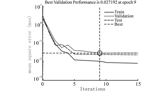
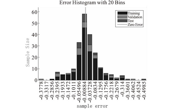

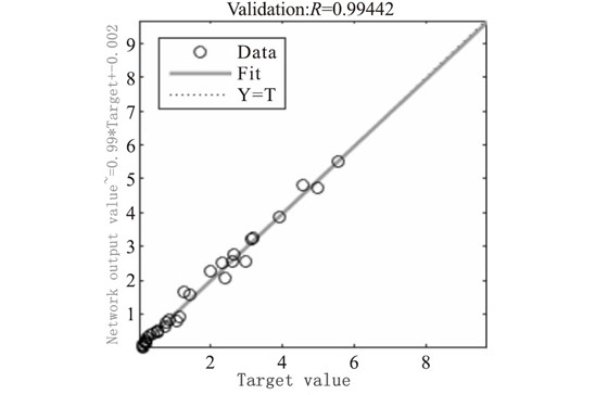
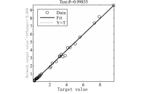
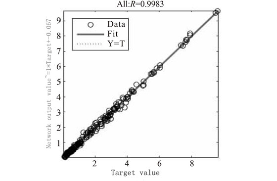
In Figure 4, the abscissa is the number of iterations, and the ordinate is the mean square error. It can be seen that the mean square error of the network dropped rapidly in the first 5 iterations, and then the rate of decline slowed down; the mean square error of the verification sample reached a minimum in the 9th iteration, and the network verified the sample's performance in the subsequent 6 iterations. The mean square error has not been reduced, so it is determined that the network generalization stops improving and the training ends. In Figure 5, the abscissa is the sample error, and the ordinate is the number of samples. It can be seen that most of the sample errors are distributed near the error zero point, and are basically normally distributed, and the network fits well. In Figure 6, the abscissa is the target value, and the ordinate is the network output value. It can be seen from the figure that the output value of the network is basically the same as the target value. The data points are all near the regression line and are evenly distributed on both sides. The network fits well. The prediction model was used to predict the radial force Fp, the tangential force Fc, the axial force Ff and the surface roughness Ra of the test group, and the relative errors were calculated respectively. The average relative errors and the prediction accuracy after sorting are shown in Table 8. The results show that the BP neural network based on the L-M optimization algorithm has a good fitting and predicting effect on cutting force and surface roughness.
|
Predictive Object Points |
Radial force |
Tangential force |
Axial force |
surface roughness |
|
Error |
8.99 |
3.14 |
9.93 |
16.57 |
| Forecast Accuracy |
91.01 |
96.86 |
90.07 |
83.43 |
Conclusion
(1) Based on the full factor test method of cutting test, the influence of cutting amount on cutting force and surface roughness in PCD tool turning of super-hard aluminum alloy and its change law are studied. The results of the study show that there is no interaction between the back-cutting amount, feed and cutting speed of PCD tool turning super-hard aluminum alloy; the back-cutting amount and cutting speed have little effect on the surface roughness; the feed rate has little effect on the surface The effect of roughness is obvious, and with the increase of feed rate, the growth rate of surface roughness shows a larger trend. It also shows that the full factor test method is used to comprehensively study the degree of influence of cutting parameters on surface roughness and its changing law. It has good application value.
(2) Established a cutting force and surface roughness prediction model based on BP neural network to predict the cutting force and surface roughness of PCD tools for turning super-hard aluminum alloy. The prediction accuracy of cutting force and surface roughness is high, which has good reference value for the research of cutting performance of new super hard aluminum alloy materials.
<< :Causes and countermeasures of tool chipping
<< :Solve the problem of processing the cylinder head valve seat conduit hole
With tungsten carbide prices soaring 200%+, PCD & CBN become cost-effective alternatives. Moresuperhard provides high-quality PCD/CBN blanks, grinding wheels & grinders to help manufacturers reduce costs and improve efficiency.
More Superhard supplies domestic 8-inch CVD diamond heat sink wafers, mass-produced in February 2026, with ultra-high thermal conductivity and excellent thermal expansion matching. Widely used in semiconductor, laser, aerospace and other fields, please call the consultation hotline for details.
Add: Zhongyuan Rd, Zhongyuan District, Zhengzhou, 450001, Henan, China
Tel: +86 17700605088